Assignment 2
Computational Photography
Alex Berg
This assignment explores image compositing and in-painting using gradient domain processing. We will begin with part I due Monday Feb 8 by midnight.
Part I
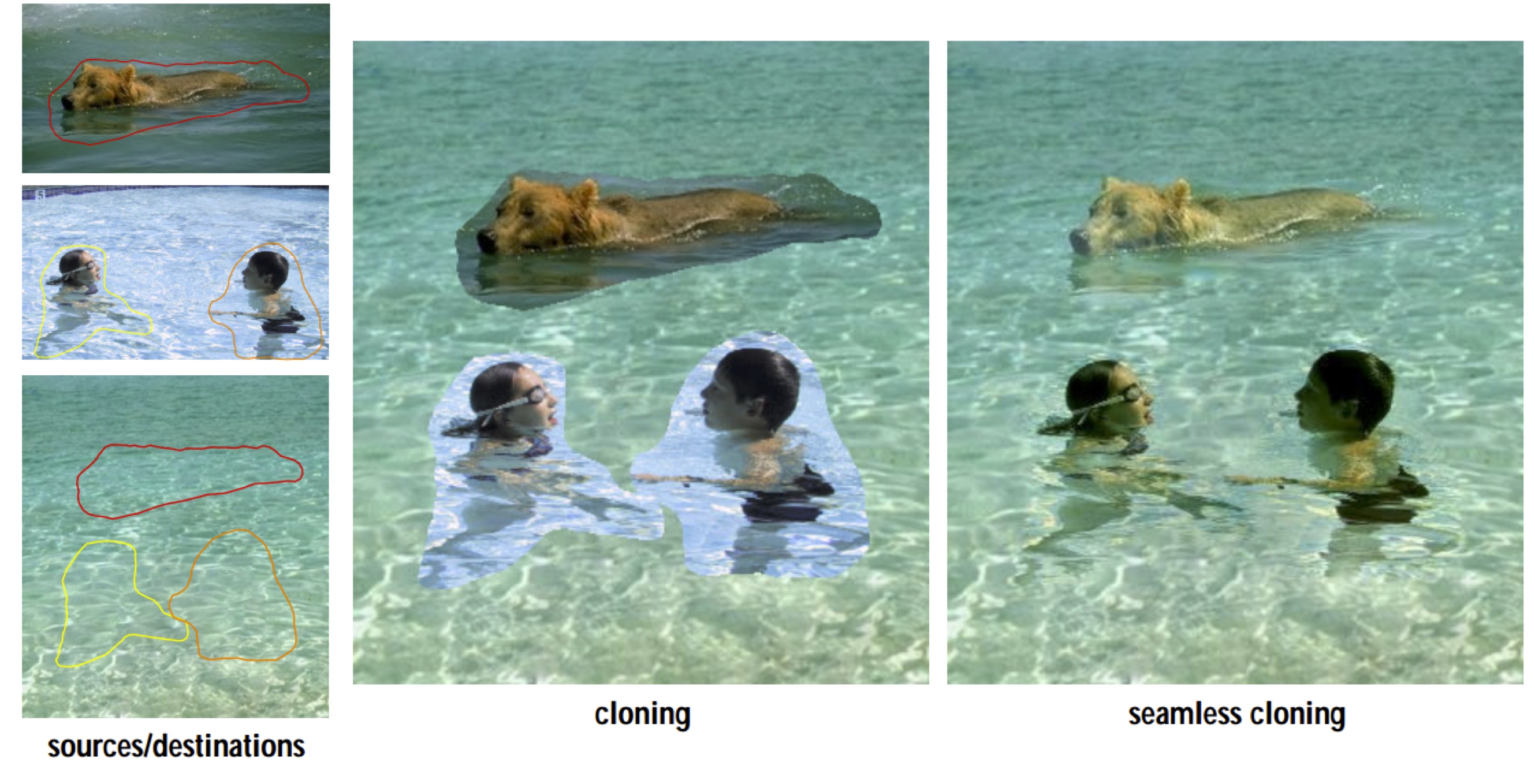
In part one you will develop code to integrate part of an image into another image, as in this example:

Click on the image to see a research paper with more detail than you need.
This will proceed in stages:
- Find two images, make a binary mask using any tool you like, and write matlab code to copy the pixels where the mask is 1 from one image into the other.2pts
- Smooth the mask and blend the images using alpha blending3pts
- Make the mask a bit larger than the region you want to insert into an image and use gradient domain editing to composite the images.10 pts toy problem + 10 points compositing images using this technique
There is a nice set of walk through slides about gradient domain editing from James Hays at Brown, here.
We can think of gradient domain editing as copying some of the gradients (derivatives in the x and y direction) from one image over some gradients of another image. The trick is reconstructing an image that has that new set of gradients as they come from two sources. This can be approached an optimization problem and solved using least-squares. The optimization takes place over the pixel values in the resulting image, and the objective function is how well the gradient of the image matches the desired gradients, and how well certain pixels in the image match some fixed pixel values. Here is a version of the optimization problem:

The idea is to optimize over the new image, N, where Ni refers to pixel i in N. So there will be one variable to find for each pixel location. The objective function that we want to minimize measures how closely the gradient in the new image match the gradients in the source image, S. We care about this inside the region where we are inserting content, R. That is the first double summation in the objective function. On the boundary of R we want to make sure the gradient between the existing pixel outside of R in the target image and the new pixel inside the region has the same gradient as the source image as well. That is the second double sum in the objective function. There are some implicit constraints that the entries in N fall into the valid range for pixel values, but in general these can be avoided, and if the solution to the unconstrained problem goes out of range (e.g. below 0) it can just be clamped at 0. You assignment is to use this technique to insert part of one image into another. You should do the following warm-up exercise first for partial credit.
Toy Problem (10 pts) [from Derek Hoiem]
 The implementation for gradient domain processing is not complicated, but it is easy to make a mistake, so let's start with a toy example. Reconstruct this image from its gradient values, plus one pixel intensity. Denote the intensity of the source image at (x, y) as s(x,y) and the value to solve for as v(x,y). For each pixel, then, we have two objectives:
1. minimize (v(x+1,y)-v(x,y) - (s(x+1,y)-s(x,y)))^2
2. minimize (v(x,y+1)-v(x,y) - (s(x,y+1)-s(x,y)))^2
Note that these could be solved while adding any constant value to v, so we will add one more objective:
3. minimize (v(1,1)-s(1,1))^2
For 10 points, solve this in Matlab as a least squares problem. If your solution is correct, then you should recover the original image.
Implementation Details
The first step is to write the objective function as a set of least squares constraints in the standard matrix form: (Av-b)^2. Here, "A" is a sparse matrix (try "help sparse" in matlab), "v" are the variables to be solved, and "b" is a known vector. It is helpful to keep a matrix "im2var" that maps each pixel to a variable number, such as:
[imh, imw, nb] = size(im);
im2var = zeros(imh, imw);
im2var(1:imh*imw) = 1:imh*imw;
Then, you can go through each pixel location and write objective 1 above as:
e=e+1;
A(e, im2var(y,x+1))=1;
A(e, im2var(y,x))=-1;
b(e) = s(y,x+1)-s(y,x);
Here, "e" is used as an equation counter. Note that the y-coordinate is the first index in Matlab convention. As another example, objective 3 above can be written as:
e=e+1;
A(e, im2var(1,1))=1;
b(e)=s(1,1);
To solve for v, use
v = A\b; (try "help mldivide" in matlab to see what this does) or
v = lscov(A, b); (similarly try "help lscov")
Then, copy each solved value to the appropriate pixel in the output image.
 The implementation for gradient domain processing is not complicated, but it is easy to make a mistake, so let's start with a toy example. Reconstruct this image from its gradient values, plus one pixel intensity. Denote the intensity of the source image at (x, y) as s(x,y) and the value to solve for as v(x,y). For each pixel, then, we have two objectives:
